The FASTA-like first step of alignment #
The
FASTA algorithm
(
Citation: Lipman & Pearson, 1985
Lipman,
D. & Pearson,
W.
(1985).
Rapid and sensitive protein similarity searches.
Science, 227(4693). 1435–1441. Retrieved from
http://www.ncbi.nlm.nih.gov/pubmed/2983426
)
can be considered as the ancestor of BLAST
(
Citation: Altschul, Gish
& al., 1990
Altschul,
S.,
Gish,
W.,
Miller,
W.,
Myers,
E. & Lipman,
D.
(1990).
Basic local alignment search tool.
Journal of molecular biology, 215(3). 403–410.
https://doi.org/10.1006/jmbi.1990.9999
)
. It has the advantage of being easy to implement. It primarily calculates the best shift to apply between the two sequences under consideration to minimize the
Hamming distance (number of differences) between them. This alignment algorithm is used in obipairing
to determine the position and the size of the overlapping region of paired-end reads. These two criteria will guide the
exact alignment method for the subsequent step, and determine the segments of the reads to align.
The FASTA-like algorithm builds a table of 4mers (DNA word of length 4) with their positions for the forward and reverse reads.
To illustrate, let us consider two short reads, A: ACGTTAGCTAGCTAGCTAA and B: CGCTAGCTAGCTAATTTGG, each of 19 nucleotides, with positions indexed from 00 to 18:
The sequences are both composed of \(19 - 4 + 1 = 16\) overlapping 4mers. An illustration of the overlapping 4mers is shown below for sequence A:
0000000000111111111
0123456789012345678

ACGTTAGCTAGCTAGCTAA

ACGT AGCT GCTA CTAA
 CGTT GCTA CTAG
  GTTA CTAG TAGC
   TTAG TAGC AGCT
    TAGC AGCT GCTA
The 4mer indices of sequences A and B can then be compared as follows:
graph LR
 %%{init: {'flowchart': {'nodeSpacing': 10, 'rankSpacing': 30, 'htmlLabels': true}} }%%
 subgraph Sequence_A
    A_ACGT:::list@{ shape: hex, label: "00"}
    A_AGCT:::list@{ shape: hex, label: "05, 09, 13"}
    A_CGTT:::list@{ shape: hex, label: "01"}
    A_CTAA:::list@{ shape: hex, label: "15"}
    A_CTAG:::list@{ shape: hex, label: "07, 11"}
    A_GCTA:::list@{ shape: hex, label: "06, 12, 14"}
    A_GTTA:::list@{ shape: hex, label: "02"}
    A_TAGC:::list@{ shape: hex, label: "04, 08, 12"}
    A_TTAG:::list@{ shape: hex, label: "03"}
end

 subgraph Sequence_B
    B_AATT:::list@{shape: hex, label: "12"}
    B_AGCT:::list@{shape: hex, label: "04, 08"}
    B_CAGC:::list@{shape: hex, label: "02"}
    B_CGCT:::list@{shape: hex, label: "00"}
    B_CTAA:::list@{shape: hex, label: "10"}
    B_GAGC:::list@{shape: hex, label: "01"}
    B_GCTA:::list@{shape: hex, label: "05, 09"}
    B_GGCT:::list@{shape: hex, label: "18"}
    B_TAAT:::list@{shape: hex, label: "13"}
    B_TAGC:::list@{shape: hex, label: "03"}
    B_TTGG:::list@{shape: hex, label: "16"}
    B_TTTC:::list@{shape: hex, label: "15"}
end


    AATT:::red --> B_AATT
    A_ACGT --> ACGT:::red
    A_AGCT --> AGCT:::green --> B_AGCT
    CAGC:::red --> B_CAGC
    CGCT:::red --> B_CGCT
    A_CGTT --> CGTT:::red
    A_CTAA --> CTAA:::green --> B_CTAA
    A_CTAG --> CTAG:::red
    GAGC:::red --> B_GAGC
    A_GCTA --> GCTA:::green --> B_GCTA
    GGCT:::red --> B_GGCT
    A_GTTA --> GTTA:::red
    TAAT:::red --> B_TAAT
    A_TAGC --> TAGC:::green --> B_TAGC
    A_TTAG --> TTAG:::red
    TTGG:::red --> B_TTGG
    TTTC:::red --> B_TTTC

    classDef green fill:#9f6, width:80px, height:50px, font-size:14px, align-items:center, text-align:center
    classDef red fill:#FF8080, width:80px, height:50px, font-size:14px, align-items:center
    classDef list stroke:#333, stroke-width:2px, width:80px, height:30px, font-size:14px
The diagram above indicates that the two sequences share four 4mers, highlighted in green.
Next, the algorithm computes \(\Delta = Pos_A - Pos_B\) for each 4mer shared between sequences A and B. If a 4mer occurs more than once, all the combinations of the differences are considered for that 4mer.
| 4mer | positions on A | positions on B | \(\Delta\) |
|---|---|---|---|
| AGCT | 05, 09, 13 | 04, 08 | 1, -3, 5, 1, 9, 5 |
| CTAA | 15 | 10 | 5 |
| GCTA | 06, 12, 14 | 05, 09 | 1, -3, 7, 3, 9, 5 |
| TAGC | 04, 08, 12 | 03 | 1, 5, 9 |
Then, for each \(\Delta\) value, the algorithm computes its frequency, as well its relative score (RelScore), expressed as the frequency of the \(\Delta\) value normalized by the number of 4mers involved in the overlap. This allows to identify the best \(\Delta\) value, i.e. the one having the highest RelScore
\[ RelScore = \frac{Frequency}{length(overlap) - (4-1)} \]| \(\Delta\) | Frequency | RelScore = Frequency/(Overlap - 3) |
|---|---|---|
| 5 | 5 | 0.455 |
| 9 | 3 | 0.428 |
| 1 | 4 | 0.267 |
| -3 | 2 | 0.154 |
| 7 | 1 | 0.111 |
| 3 | 1 | 0.077 |
The table above is the equivalent of a
DNA Dot Plot. A \(\Delta\)
value corresponds to one diagonal in the dot plot. By default, obipairing
considers the diagonal with the highest RelScore as the optimal alignment, i.e. the best shift-only alignment (no insertions or deletions allowed in the overlap).
If the --fasta-absolute option is used, the best \(\Delta\)
(or diagonal) is the one exhibiting the highest Frequency.
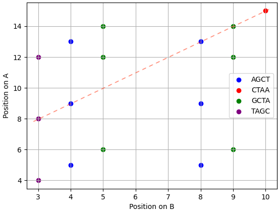
Shared 4mer positions:
This plot is a thresholded DNA dot plot of both sequences. Each point corresponds to a shared 4mer and is located at its respective positions on sequences A & B. The red dotted line indicates the diagonal with the greatest number of dots, here representing five overlapping 4mers and corresponding to a positional difference of 5 between sequences.
In this example, the diagonal having the largest RelScore (0.455) corresponds to a \(\Delta\) value of 5, which was observed five times. Thus, the sequence similarity between the sequences A and B is maximized by shifting B of 5 positions relatively to A.
Sequence A: ACGTTAGCTAGCTAGCTAA-----
Sequence B: -----CGCTAGCTAGCTAATTTGG
Overlap   :      .+++++++++++++
This delimits the overlapping region between the two reads.
References #
- Altschul, Gish, Miller, Myers & Lipman (1990)
- Altschul, S., Gish, W., Miller, W., Myers, E. & Lipman, D. (1990). Basic local alignment search tool. Journal of molecular biology, 215(3). 403–410. https://doi.org/10.1006/jmbi.1990.9999
- Lipman & Pearson (1985)
- Lipman, D. & Pearson, W. (1985). Rapid and sensitive protein similarity searches. Science, 227(4693). 1435–1441. Retrieved from http://www.ncbi.nlm.nih.gov/pubmed/2983426